import matplotlib.pyplot as plt
import matplotlib.image as mpimg
import numpy as np
%matplotlib inline
# we will be using linear algebra functions from numpy.linalg
import numpy.linalg as la
Noise-based Textures
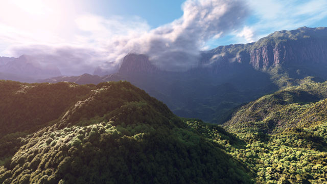
Computer graphics often uses procedural techniques to generate highly detailed visuals. For example, the terrain shown below would be very difficult for an artist to generate by hand. Instead, most of the work is done by code using something called Perlin noise to create a highly detailed natural appearance.

Invented by Ken Perlin in 1982 while working on the movie Tron, Perlin noise uses randomness and repetition to synthesize 2D and 3D textures. In 1997, Perlin won an Academy Award for Technical Achievement from the Academy of Motion Picture Arts and Sciences for this contribution to graphics. Perlin noise and techniques based off of it are still widely used in games and movies today.
Today, we will write some code to simulate a 2D smoke texture. We won't be using Perlin's function...instead we will do something less efficient but easier to implement.
The first step is to create a greyscale image represented by a numpy array with the all of the color channels having 0.5 as an initial value.
After that we will repeatedly, randomly generate a line that partitions the pixels of the image. On one side of the line we will increase the brightness of each pixel by some value colorDelta. On the other side, we decrease the pixel brightness by colorDelta. After enough iterations, you should see something resembling a smoke texture.

Create the initial image
Create the numpy array initialImage with shape (width, height, 3), where all entries have the initial value 0.5
plt.imshow(initialImage)
Understanding the algorithm
You will randomly generate a point p and a unit vector n that is perpendicular to the line that partitions the domain.
Suppose now you take another random point b inside the domain, and obtain the distatnce from p to b. If you take the dot product of this distance with the unit vector n and you get a positive scalar, then you are on one side of the domain (in the illustration below the orange side), and if you get a negative scalar, you are on the other side (the green area in the illustration below).

Generate a random float point inside the domain of the image (here a $100 \times 100$ square), and store it in the variable pt.
Generate the random unit vector n, that is perpendicular to the line that splits the image.
Generate another random float point inside the domain, and store it as the variable a.
You can now write the vector from pt to u, and then get use the dot product to determine which side of the domain point a is.
dist = a - pt
dist@n_vec
Write a code snippet that goes over all the points inside the domain ($x \in [0,width]$ and $y \in [0,height]$). Your code should start by initializing your noiseImage as a copy of the initialImage. Then if the point gives a positive scalar value from the dot product, increase the current pixel value in noiseImage by 0.01, otherwise, decrease the current pixel value by 0.01.
noiseImage = np.copy(initialImage)
plt.imshow(noiseImage)
Time to run the numerical experiment above several times (start with N = 10 and increase to 100 and 500 once you are confident your algorithm is working properly). Each numerical experiment should start with random pt and n vectors.
noiseImage = np.copy(initialImage)
N = 500
plt.imshow(noiseImage)
Spot the difference!
In this next example, you will write a code snippet that finds the differences between two images. First we will load the image, a png with the 4 rgba channels:
img = mpimg.imread('pikachu.png')
plt.imshow(img)
print(img.shape)
And we can get a gray scale version of the image (same that you did on week 3)
BW_img = np.sum(np.array(img), axis=-1).astype(np.float32)/(3*255)
print(BW_img.shape)
We want to spot the differences between the two images. Let's first split the above figure in two images:
image1 = BW_img[:,:392]
image2 = BW_img[:,-392:]
ly = image1.shape[0]
lx = image1.shape[1]

fig = plt.figure(figsize=(10,10))
fig.add_subplot(121)
plt.imshow(image1, cmap="gray")
plt.title('Image 1')

fig.add_subplot(122)
plt.imshow(image2, cmap="gray")
plt.title('Image 2')
Write a code snippet that compares both images as follows:
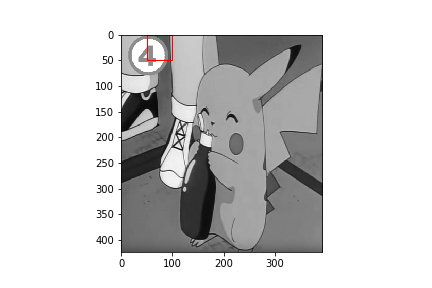
1) take subimages of images1 and image2 defined by a $50 \times 50$ square, as illustrated below:
2) take the difference between these subimages - note this difference is still a 2d array
3) choose a scalar measurement that quantifies the difference between the subimages. For this part, we suggest using the 2-norm (if you don't know what this is, don't worry, we will talk about norms in CS357 class very soon!)
numpy.linalg.norm(2darray,2)
4) you now have a measurement of the error between the two subimages. If $error > 0.01$, you should add a square to the image, marking the region where you spotted the difference
You can use what your learned in week 3 to add rectangles to an existing image (and use fill=False)
