!pip3 install pygraphviz

import numpy as np
import numpy.linalg as la
import matplotlib.pyplot as plt
import graph

Graphs and Algebraic Graph Theory¶

In graph theory, a graph is a set of nodes ("vertices") that are connected to one another with edges.

(https://en.wikipedia.org/wiki/Graph_(discrete_mathematics)#/media/File:6n-graf.svg)

Graphs are general enough to be used in many different applications: they can represent connections between friends on social networks or roads and intersections when looking at maps (calculating turn-by-turn directions involves solving a graph problem!).

Adjacency Matrix¶

As almost everything else in Linear Algebra, we can represent a graph using a matrix. For a graph that has $n$ nodes, you will have the adjacency matrix ${\bf A} \in \mathbb{R}^{n \times n}$ such that:

$${\bf A}_{i,j} = \begin{cases} 1 & \text{if node } i \text{ connects to node } j \\ 0 & \text{otherwise} \end{cases}$$

So we must have some strict ordering to the nodes in order to create this matrix. We can think of this as the columns of ${\bf A}$ represent incoming edges, while the rows of ${\bf A}$ represent outgoing edges. So for example, entry ${\bf A}_{0,2}$ would store information on if node $0$ connects to node $2$.

Below is a small example.

adj_matrix = np.array([[0, 1, 0],
                       [1, 0, 1],
                       [0, 1, 0]])

Stop reading, and first sketch the graph corresponding to the matrix above.

Because here for each connected pair of nodes $(i,j)$ we also have that $(j,i)$ are connected, the matrix is symmetric along the diagonal. This is called an undirected graph because edges do not have direction. For the adjacency matrix ${\bf A}$ of an undirected graph, we thus have that ${\bf A}^T = {\bf A}$.

You can use the function graph.draw_matrix to check if your sketch is correct.

graph.draw_matrix(adj_matrix, show_weights=False)

Here is a slightly more interesting example. Any nonzero values along the diagonal are called "self loops".

A = np.array([[0, 1, 1, 0],
              [1, 0, 0, 1],
              [1, 0, 1, 0],
              [0, 1, 0, 1]])

graph.draw_matrix(A, show_weights=False)

Take a few moments to understand how the structure of the graph relates to the matrix given above (and vice versa).

Graph Walks¶

In graph theory, a "walk" of size $k$ is a sequence of $k$ vertices and $k-1$ edges between two nodes (including the start and end) that may repeat. You can imagine it as the path taken if you were to literally "walk" from one node to another in $k-1$ steps.

Hence the adjacency matrix ${\bf A}$ tells us where we can go in one step (a walk of size $2$). Let's take another look at the above example:

A = np.array([[0, 1, 1, 0],
              [1, 0, 0, 1],
              [1, 0, 1, 0],
              [0, 1, 0, 1]])

graph.draw_matrix(A, show_weights=False)

In this example, observe that from node $1$, we can either "walk" to node $0$ or $3$ in one step. Indeed, row $1$ has value of $1$ in columns $0$ and $3$, and $0$ otherwise.

Knowing this, if the adjacency matrix ${\bf A}$ tells us where we can go in one step (a walk of size $2$), what does the matrix product ${\bf A A}$ tell us?

A @ A

Now entry $\left({\bf A}^2\right)_{ij}$ tells us if we are able to get from node $i$ to node $j$ in 2 steps (a walk of size $3$), and how many different walks you can take to get there as well.

Discuss the following questions with your group:

Which nodes can be reached from node $1$ in 2 steps?
How many different walks of size $3$ are possible from node $2$ to node $1$?
Use the function graph.draw_matrix to plot $\left({\bf A}^2\right)$. You can use the attribute show_weights=True. How does this depiction reflect your previous answers?

Note that $\left({\bf A}^2\right)_{0,1}$ tells us node $0$ is not connected to node $1$ because we can no longer reach it in exactly $2$ steps.

For the given adjacency matrix ${\bf A}$ above, what if we are interested in finding some node in up to $k$ steps? The issue here is that if a node is reached in $ n < k $ steps, we are forced to move off of it at the next step. Can you modify the graph such that calculating the matrix project ${\bf A}^k$ will tell us if a node is reachable in $1 \leq n \leq k$ steps?

Hint: If we reach the desired node early, how can we adjust the graph so that we can remain there until step $k$? Can we leverage self-loops here?

# Set M to be the new, modified matrix
M = ...

Lets try a walk of $3$ steps (size $4$).

la.matrix_power(M, 3)

which is the same as:

M@M@M

Because each entry is nonzero, we can start from any node and reach any other node in at most 3 steps.

Number of Steps in Walk¶

In the previous examples we were picking arbitrary values of $k$ for our walks, but what is the optimal (least) value of $k$ to check if any node can reach any other node? How might your answer change if you know that the graph is fully connected (i.e. each node is connected to every other node)?

Let's look at a few scenarios here. Here is the "optimal" graph, where each node is directly connected to every other one:

n = 4
A = np.ones((n, n))
graph.draw_matrix(A, show_weights=False)

A

We don't even need to perform the matrix multiplication to know that the optimal value is 1 step ($k=2$). Let's look at the opposite case where each node is connected to at most two other nodes:

n = 6
A = np.eye(n, k=-1) + np.eye(n, k=1)
print(A)

You can take a look at the numpy.eye documentation to see how we can use the argument k to define upper and lower diagonals.

graph.draw_matrix(A, show_weights=False)

As before, create the matrix M such that each node can also move to itself.

Now, determine the value of $k$ that tells us if all nodes can reach any other node.

At this point, just try different values. Once you find one that works, you may be able to make some conclusions.

How is the value of $k$ related to the number of nodes?

k = 2 # <-- what should k be?
Mk = la.matrix_power(M, k-1)
graph.draw_matrix(Mk, show_weights=False)

Therefore, this value of $k$ is the maximum value needed to determine if any graph is connected. We can use this to determine connectivity of graphs.

Disconnected Graphs¶

So what do the powers of the adjacency matrix look like for graphs with disjoint parts?

A = np.array([[0, 1, 0, 0, 0],
              [1, 0, 0, 0, 0],
              [0, 0, 0, 1, 1],
              [0, 0, 1, 0, 1],
              [0, 0, 1, 1, 0]])

graph.draw_matrix(A, show_weights=False)

Here we have a graph with two "groups" of nodes that are connected to each other. These are called "connected components".

Now run a walk of size $k$, using the maximal necessary value of $k$ that you have determined previously. Modify the matrix as usual to allow for self loops. Print and examine the values of ${\bf A}^{k-1}$. You may also want to visualize your result using graph.draw_matrix.

Notice how we get two distinct "components" in the matrix that correspond with the two visible components in the graph itself.

Lets look at another example of a graph of $n=10$ nodes.

n = 10
A = np.array([[0, 1, 0, 1, 0, 0, 0, 0, 0, 0],
              [1, 0, 0, 0, 0, 0, 0, 0, 0, 0],
              [0, 0, 0, 0, 1, 0, 0, 0, 1, 0],
              [1, 0, 0, 0, 0, 0, 0, 0, 0, 0],
              [0, 0, 1, 0, 0, 0, 0, 0, 0, 0],
              [0, 0, 0, 0, 0, 0, 0, 0, 1, 0],
              [0, 0, 0, 0, 0, 0, 0, 1, 0, 1],
              [0, 0, 0, 0, 0, 0, 1, 0, 0, 1],
              [0, 0, 1, 0, 0, 1, 0, 0, 0, 0],
              [0, 0, 0, 0, 0, 0, 1, 1, 0, 0]])
graph.draw_matrix(A, show_weights=False)

Create the matrix M as usual from the adjacency matrix, and create Z such that ${\bf Z} = {\bf M}^{k-1}$ with maximal value of $k$ as above.

Now we can plot each entry of ${\bf Z}$ to see the connectivity. The function plt.spy() will display all non-zero values of the matrix as black squares.

Z

plt.spy(Z)

You may see some repeated rows and columns, these are the "connected components" since every node can move freely to each other in them. Note that the actual weight (value of the matrix entry) is not relevant here. We are just interested to know the non-zero pattern (which represents the connectivity). For that reason, we can redefine Z as:

Z = (Z>0).astype(int)
Z

We find the unique rows/column to see how many unique components we have and which nodes they occupy.

We use the function numpy.unique to return the unique rows of the 2d array Z using the attribute axis=0.

components = np.unique(Z, axis=0)
plt.spy(components)

The three unique rows are the three unique components, and by examining the columns we can see which nodes occupy the components.

graph.draw_matrix(Z, show_weights=False)

Social Network Analysis¶

One interesting application of graphs is exploring how people are friends with each other on social media, a process called social network analysis. By modeling people as nodes and connecting them with edges if they are friends, we can model several properties of the network.

(http://www.kakadu-works.com/myfnetwork/welcome.html)

Let's imagine we have a random subset of $50$ people, some of whom are friends with each other, and we would like to determine groups of friends within the social network. The function below will create your matrix representing the social network.

n = 50
A = graph.gen_random_friends(n)

We have fairly sparse adjacency matrix connecting people to each other, here we will consider "friend of a friend" and so on to be the same friend group.

plt.spy(A)

We can also visualize in a graph format:

graph.draw_matrix(A, show_weights=False)

Now we need to find all the separate friend groups. Because we are defining friend groups as including "friends of friends", we just need to find the connected components!

As you have done before, find all the connected components of the graph. Plot all unique rows of the connectivity matrix.

What is the number of friend groups? How many people are in the largest friend group? Print these values out.

Hint: To determine the size of the largest friend group, first find a way to compute the sizes of the friend groups. Then, find the largest of those values.

Meme Spread¶

Lets examine a slightly different problem. If we are given a friend graph as we have above, how many people will receive a meme assuming each person sends it to all of their friends?

(Meme stolen from [reddit.com/r/mathmemes](https://www.reddit.com/r/mathmemes/comments/f9qvhm/linear_algebra_in_nutshell/))

We will use a slightly larger graph of $n=100$ people.

n = 100
A = graph.gen_random_friends(n, 0.985)
plt.spy(A)

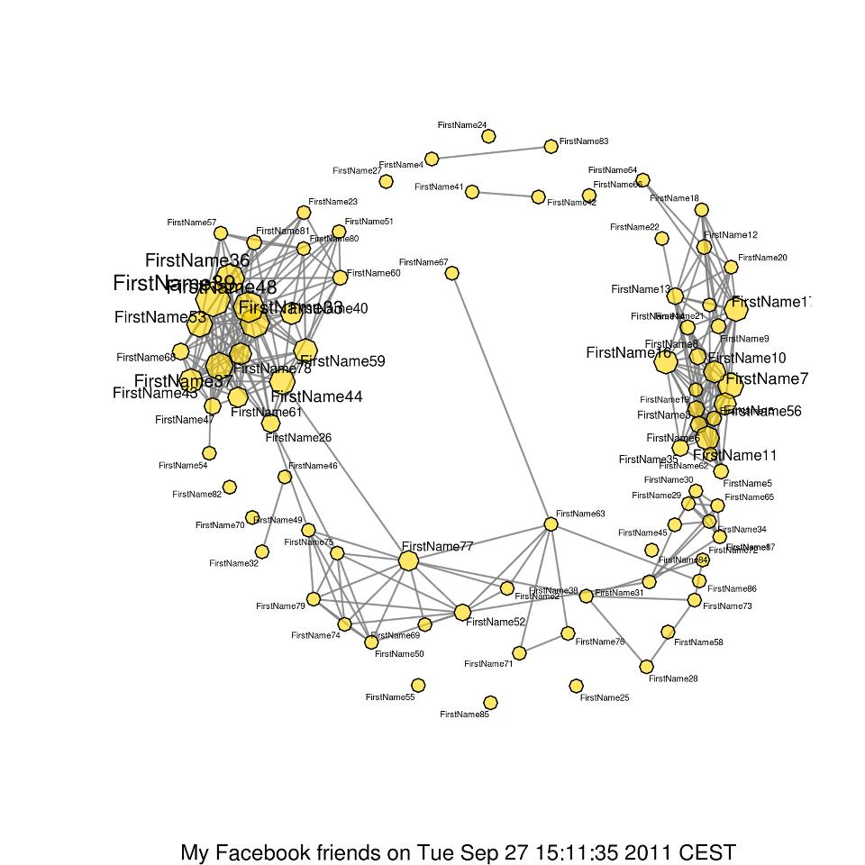
Here is the (quite large!) graph showing friend connectivity:

graph.draw_matrix(A, show_weights=False)

Suppose the meme was created (or reposted) by person 50, (the $51^{st}$ row/column of the adjacency matrix). By simulating walks through the graph, we can determine who will receive the meme if everybody sends it to all of their friends.

Determine and print the number of people that will receive the meme when starting at person 50. Recall that the connectivity matrix (some power of the adjacency matrix) will contain a non-zero value for each pair of nodes that are connected.

Confirm your answer with the graph above, depending on how many friends person 50 has (or doesn't have) this could be an interesting value.

Optimize our meme spread by trying to find the initial person who will give us the largest "spread". Identify the person who will spread the meme to the most people, and print the number of people that will receive it. Note that there may be multiple "best" people: for tie-breaking, take the person with the smallest assigned index (i.e. take person $2$ over person $5$ if they both yield the maximum spread).